CS6670 Project 1: Feature Detection and Matching

Peng Chen (pc423)

1. Feature Detection

1. 1. Harris Corner Detection

In this step, we try to identify points of interest in the image using the Harris corner detection method.  The steps are as follows, for each point in the image, consider a window of pixels around that point.  Compute the Harris matrix H for that point, defined as

where the summation is over all pixels p in the window.  The weights should be chosen to be circularly symmetric (for rotation invariance).  Her we use 5x5 Gaussian mask.

Compute the corner strength function in order to find interest points

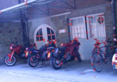
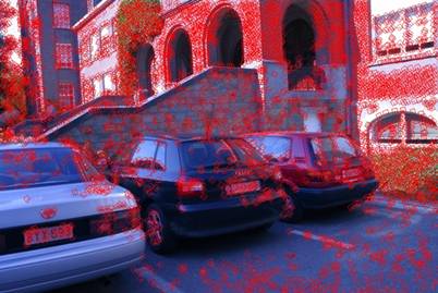
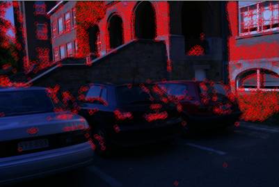
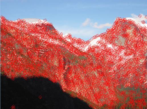
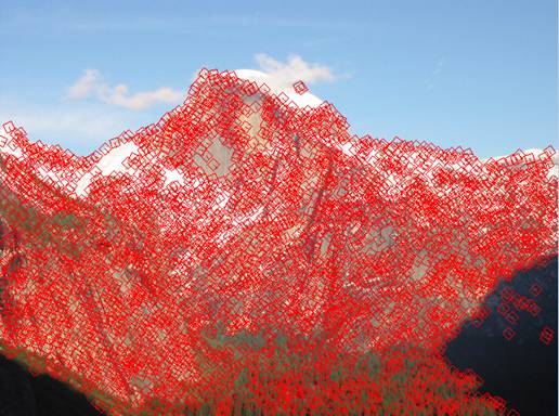
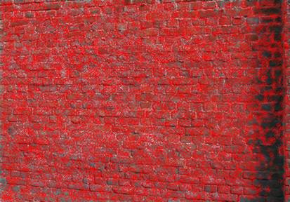
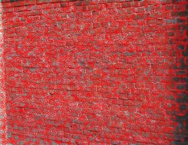
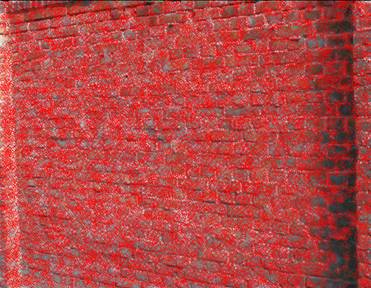
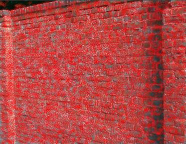
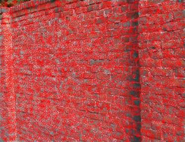
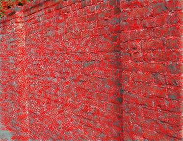
Choose c = 0.01 as a threshold. The interest point is a local maximum in a 5x5 local window. The orientation can be computed by two methods, the first one is finding the eigenvector which corresponds to the largest eigenvalue of the Harris Matrix, while the second one is simply using the gradient at that point as its orientation. Here the second method is used.

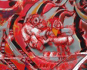
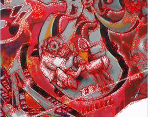
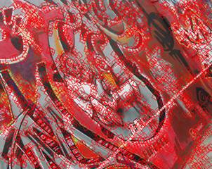
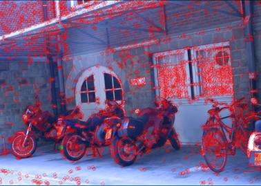
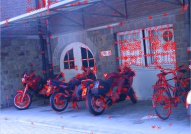
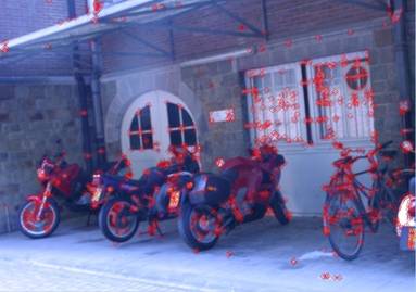
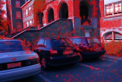
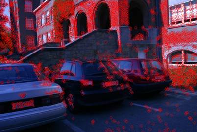
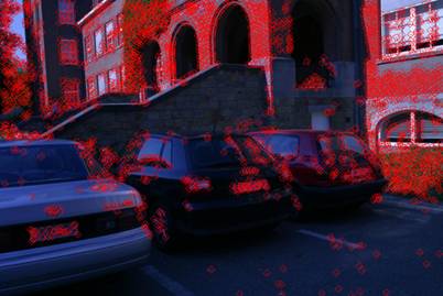
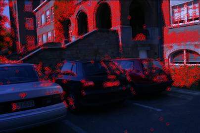
Below list all the example images with orientated features detected by using Harris corner detector.

1.2. Adaptive Non-Maximal Suppression

Here, we try to implement an Adaptive Non-Maximal Suppression detector to select a fixed number of feature points from each image. Interest points are suppressed based on the corner strength f_HM and only those that are a maximum in a neighbourhood of radius r pixels are retained. Conceptually, we initialize the suppression radius r = 0 and then increase it until the desired number of interest points nip is obtained.

In practice, we can perform this operation without search as the set of interest points that are generated in this way form an ordered list. The first entry in the list is the global maximum, which is not suppressed at any radius. As the suppression radius decreases from infinity, interest points are added to the list. However, once an interest point appears, it will always remain in the list. This is true because if an interest point is a maximum in radius r then it is also a maximum in radius r′ < r. In practice we robustify the non-maximal suppression by requiring that a neighbor has a sufficiently larger strength. Thus the minimum suppression radius r_i is given by

Parameters

· robust parameter c = 0.9

· interest point number n_i

Experiments:

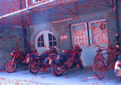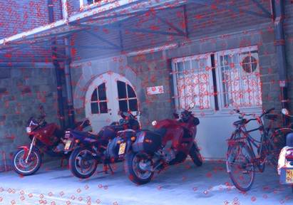
                                          n_i =2000                                                                                               n_i =1000

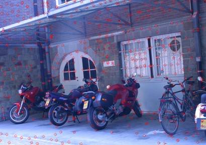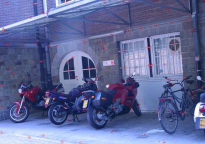
                                          n_i =500                                                                                                   n_i =100

2. Feature Description

2. 1 simple descriptor

The simple descriptor is simply using a 5x5 square window centered at the feature point. It is a fairly good descriptor without losing any information, and is translation invariant. By normalizing the descriptor, it is also possible to achieve more or less illumination invariance.

2. 2 MOPS descriptor

Given a feature point, the descriptor is formed by first sampling a 41x41 patch centered at that point with feature orientation, and then scaling to 1/5 size by using prefiltering. Rotating the window to horizontal and sample an 8x8 square window centered at the feature point. Finally, all the intensities in the window should be normalized by subtracting the mean, dividing by the standard deviation in the window.

2. 3 pyramids descriptor

Here I design my own descriptor based on MOPS descriptor and Gaussian Pyramids. The details for this descriptor are illustrated as follows: given a feature point, the descriptor is formed by first sampling a 32x32 patch centered at that point with feature orientation, rotating the window to horizontal, and then use Gaussian pyramids techniques, filtering the image and subsampling from the window. Finally, we can obtain a pyramid of 1x1, 2x2, 4x4, 8x8, 16x16, 32x32 images to describe the feature window, in order to save the memory, we can just use a four-level pyramid which consists of 1x1, 2x2, 4x4, 8x8 images as our descriptor. Note that all the intensities in the window should be normalized at each step. Since this descriptor combines the MOPS descriptor and Gaussian Pyramids, it definitely has certain invariant property of scale and orientation.

3. Feature Matching

3. 1 Discussion of matching performance

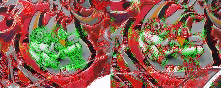
Below is an example of a feature matching for the graf image1 and image2, here we use MOPS descriptor and SSD matching algorithm. From the figure, we can see that some of the features are matched correctly, but there are still a lot of features which are matched wrongly. Comparing this with the result form the solution EXE provided by our nice TA, I find it doesn’t have a better performance than my result. So I think maybe the problem comes from the limitation of the algorithm.

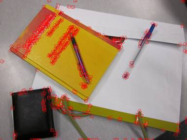
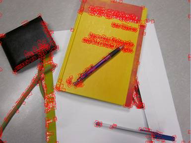
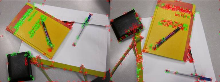
And also, I apply the above feature matching algorithm on some new photos of my own, the result is not very good but acceptable.

3. 2 ROC curves

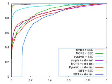
The ROC curves for the Yosmite and graf image are given below. I don’t know why we get a strange curve for the Pyramid descriptor by SSD matching algorithm, I guess one possible explanation could be pyramid descriptor is not very valid since it takes a pyramid structure as the descriptor, there could have some error during the blurring and downsampling process, or there are some bugs within my code. Put this aside, all the rest curves seem reasonable. From the figures, we can see that SIFT gives the best performance, MOPS descriptor gets the second place, then the simple descriptor and finally the Pyramid descriptor.

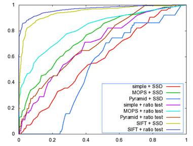
                                           Yosmite                                                                                       graf

The AUC for the above two sets of images is listed as follows:    

                            Yosmite                   graf     

Simple + SSD      0.856546              0.573946

MOPS + SSD      0.895013              0.750359

Pyramid + SSD   0.776117              0.514259

Simple + SSD     0.880455               0.689292

MOPS + SSD     0.968327               0.821569

Pyramid + SSD   0.777719              0.463625

3. 3 AUC report

Below is the average AUC report for the feature detecting and matching code for the four benchmark set: graf, leuven, bikes and wall. The data structure in the following table is Average error \ Average AUC.

Here the match type is chosen to be the SSD matching algorithm.

                           Simple 5x5                                        MOPS                                       Pyramid

graf               310.366462 \ 0.444394                287.322149 \ 0.551560                322.442096 \ 0.441408

bikes             406.212494  \ 0.545069               320.415199 \ 0.634450                 405.219651 \ 0.580645

leuven          252.282998 \ 0.571142                152.141518 \ 0.639556                361.305100 \ 0.554103

wall              351.717449 \ 0.587851                264.383011 \ 0.558100                 399.127817 \ 0.429698

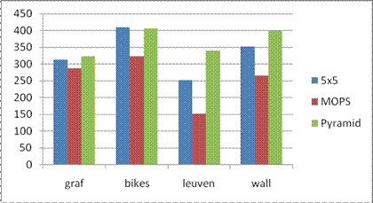
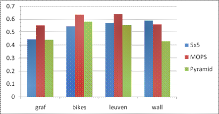
Here the match type is chosen to be the ratio matching algorithm.

                           Simple 5x5                                        MOPS                                       Pyramid

graf         310.366462 \ 0.516806                    287.322149 \ 0.574530               322.442096 \ 0.483622

bikes       406.212494 \ 0.540433                    320.415199 \ 0.650844               405.219651 \ 0.512910

leuven     252.282998 \ 0.607109                    152.141518 \ 0.738877               361.305100 \ 0.535885

wall         357.362414 \ 0.586120                    264.383011 \ 0.649671               399.127817 \ 0.438152

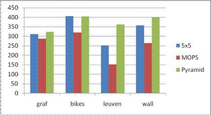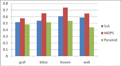
Note here, for the graf result, since the code cannot run with only three images, I downloaded the graf data from the internet and used them instead of the provided data to get the average AUC result.

4. Summary

In this project, we successfully implement the Feature detection, Feature description, Feature matching and ROC plot via different methods. And we test our program by using the provided data set and my own photos, the outcomes are completely acceptable. But unfortunately, my own designed descriptor- the Pyramid descriptor – doesn’t meet the expectation, it performs even worse than the simple descriptor. So I think pyramid descriptor is not a good candidate for the descriptor.

Reference

[1] David G.Lowe, "Distinctive image features from scale-invariant keypoints", International Journal of Computer Vision, 60, 2 (2004), pp. 91 - 110

[2] M.Brown, R. Szeliski and S. Winder, "Multi-Image using multi-scale oriented patches", International Conference on Computer Vision and Pattern Recognition 2005, pages 510 - 517

[3] K. Mikolajczyk and C. Schmid, "Indexing based on scale invariant interest points", International Conference on Computer Vision 2001, pp 525-531

[4] K. Mikolajczyk and C. Schmid, "Scale & Affine interest point detectors", International Journal of Computer Vision 60(1), 63-86, 2004